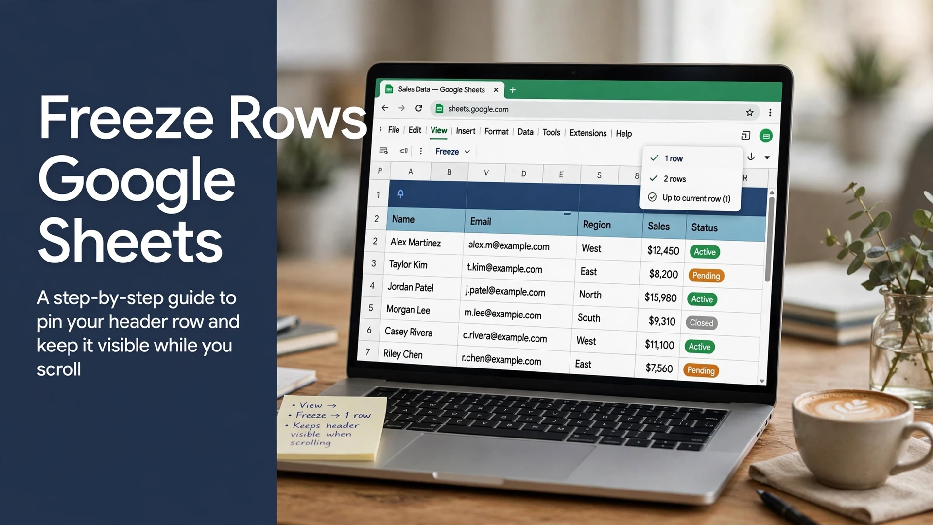
How to Freeze Rows in Google Sheets (3 Ways, Including the Drag Trick)

Quick answer: To freeze rows in Google Sheets on desktop, go to View > Freeze and pick 1 row, 2 rows, or Up to current row — or drag the thick gray handle in the sheet’s top-left corner downward. To unfreeze, use View > Freeze > No rows. On the mobile app, tap a row number and choose Freeze from the menu.
Scrolling through a long spreadsheet only to lose your column headers at the top of the screen is one of the most quietly maddening things in Google Sheets. The fix takes about five seconds: freeze the rows you want pinned, and they stay locked in place while the rest of the sheet scrolls underneath them.
I verified every method below against Google’s current Sheets interface in October 2026 (web app in Chrome on Windows 11 24H2, plus the Sheets app on Android and iPhone), and cross-checked the menu paths against Google’s official Docs Editors help pages. There are three desktop methods plus the mobile path — use whichever fits how you work.
Method 1: Freeze Rows From the View Menu (Desktop)
This is the most reliable method and the one I recommend if you want precision. The menu options tell you exactly what will happen before you click.
To freeze the top row:
- Open your spreadsheet in Google Sheets.
- Click View in the top menu bar.
- Hover over Freeze.
- Click 1 row. A thicker gray divider line appears under row 1 — that’s your frozen header.
To freeze two or more rows:
- Click any cell in the last row you want frozen. For example, click a cell in row 3 to freeze rows 1 through 3.
- Go to View > Freeze.
- Choose Up to row 3 (the label shows the row of your selected cell, so you can double-check before clicking).
If you only need the first two rows, there’s also a one-click 2 rows option in the same submenu.
Method 2: Drag the Freeze Handle (The Fastest Way)
Google Sheets hides a small drag handle in the top-left corner of the grid — the empty box sitting above row number 1 and to the left of column letter A. If your mouse is already there, this is the fastest freeze of all.
- Hover your cursor over the bottom edge of that top-left corner box (the thick gray line just above row 1). Your pointer changes into a small hand.
- Click and drag the line downward, below the last row you want frozen.
- Release. A darker divider line now separates your frozen rows from the rest of the sheet.
This does exactly the same thing as the View menu — you can confirm that afterward by opening View > Freeze and seeing the matching option checked. To undo it, drag the handle back up to the corner.
Method 3: Freeze Rows Without Touching the Mouse (Keyboard)
Here is the honest caveat: Google Sheets has no dedicated keyboard shortcut for freezing rows — Google’s official shortcuts list doesn’t include one. But you can still do it keyboard-only by opening the View menu first:
- Chrome on Windows: press Alt + V to open the View menu.
- Other browsers on Windows: press Alt + Shift + V.
- Mac: press Ctrl + Option + V.
From there, use the arrow keys to move down to Freeze, press the right arrow, arrow down to the option you want (1 row, 2 rows, or Up to current row), and press Enter. It’s not one keystroke, but once the muscle memory lands it takes about three seconds.
All Three Methods Compared
| Method | Best for | Where it lives | Note |
|---|---|---|---|
| View menu | Precision — freezing an exact number of rows | View > Freeze > 1 row / 2 rows / Up to current row | Most reliable; the “Up to row X” label confirms your selection first |
| Drag handle | Speed — your hand is already on the mouse | Top-left corner of the grid, drag down | Cursor turns into a hand when you’re in the right spot |
| Keyboard | Mouse-free workflows | Alt+V (Chrome/Windows), Ctrl+Option+V (Mac), then arrows | No single-key shortcut exists — it’s a menu walk |
| Mobile app | Quick checks on the go | Tap row number > menu > Freeze | Android and iPhone; see the steps below |
How to Unfreeze Rows in Google Sheets
Changed your mind, or froze the wrong rows? Two ways back:
- Menu method: go to View > Freeze > No rows. This unfreezes everything at once — there’s no “unfreeze just one” option, so re-freeze afterward if needed.
- Drag method: hover over the frozen divider line until the cursor turns into a hand, then drag it back up to the top-left corner.
How to Freeze Rows in the Google Sheets Mobile App (Android & iPhone)
The mobile app doesn’t have a View menu, so the gesture is different — but it works on both Android and iPhone:
- Open the spreadsheet in the Google Sheets app.
- Tap and hold the row number of the last row you want frozen (or tap it, then tap it again to open the menu).
- A small menu pops up — tap the three dots to expand it if needed.
- Choose Freeze.
This freezes rows 1 through the row you selected. To unfreeze on mobile, tap the row number again and choose Unfreeze from the same menu.
Bonus: Freeze Rows and Columns at the Same Time
Freezing isn’t limited to rows. If you also have an ID column (names, product codes) you want pinned while scrolling horizontally, you can freeze both axes — Google handles them as independent settings, so one doesn’t cancel the other:
- Go to View > Freeze and pick your rows (e.g. 1 row).
- Go to View > Freeze again and pick your columns (e.g. 1 column).
The same drag trick works for columns too: grab the left edge of the top-left corner box and drag it right.
Frozen Rows Not Working? Fixes
A few gotchas I’ve seen people hit:
- The Freeze option is grayed out. You almost certainly have view-only access to the sheet. Freezing is a change to the sheet’s layout, so you need edit permission. Ask the owner to change your role.
- Frozen rows don’t appear in your printout or PDF. That’s by design — freezing only affects on-screen scrolling, never the printed page. If you want headers repeated on every printed page, that’s a separate setting under File > Print > Headers & footers.
- You froze the wrong rows. Go to View > Freeze > No rows and start over — there’s no harm in unfreezing.
- You want to freeze rows in the middle of the sheet. Not possible — freezing always pins rows starting from row 1. Rearrange your sheet so the header rows sit at the top, or combine a frozen header with a filter to focus on the rows you care about.
FAQs
There is no dedicated keyboard shortcut for freezing rows. The fastest keyboard path: press Alt + V (Chrome on Windows) or Alt + Shift + V (other browsers) to open the View menu, then use the arrow keys to reach Freeze and pick 1 row. On a Mac, press Ctrl + Option + V.
Freezing always pins rows starting from row 1 — Google Sheets does not let you freeze rows in the middle of a sheet. If your headers aren’t at the top, move them there first (select the rows, drag them up) or use a filter instead.
Go to View > Freeze > No rows to unfreeze everything at once, or hover over the frozen divider line until the cursor turns into a hand and drag the handle back up to the top-left corner.
No. Freezing only controls which rows stay on screen while you scroll — it doesn’t change cell contents, formulas, or cell addresses. It’s a pure display aid.
Yes. Tap and hold the row number of the last row you want frozen, tap the menu (three dots if it doesn’t appear immediately), and choose Freeze. Tap the row number again and choose Unfreeze to reverse it.
Yes. Freezing rows and columns are independent settings in Google Sheets. Go to View > Freeze and set your rows, then open View > Freeze again and set your columns. Both stay pinned while you scroll.
Final Thought
Freezing rows is one of those tiny Google Sheets skills that pays for itself every single day — a frozen header row turns a 500-row export from a guessing game into a readable table. If you found the drag handle new, try it once; most people never go back to the menu. And if you’re building longer spreadsheet workflows, pair a frozen header with a filter and you’ve got a surprisingly capable little database. For capturing what you’ve built, here’s how to take a scrolling screenshot on Windows 11 so the whole sheet fits in one image.